Tutorial: Estimating health impacts of the Volkswagen emissions scandal
This blog post contains a step-by-step example of how to create an emissions scenario and use the InMAP model to estimate the resulting health impacts.
1. Introduction
The Volkswagen emissions defeat device was exposed in September 2015, when the Volkswagen Group of America (VW) admitted to violating the Clean Air Act (CAA) by installing emissions control system "defeat devices" designed to circumvent emissions tests1. The United States Environmental Protection Agency had found that the affected VW vehicles output NOx emissions at rates up to 40 times more than the EPA standard during on-road emissions testing. A couple of researchers have published the estimated exposure and health impact of the excess pollution emissions caused by the defeat devices. Several different chemical transport models were used in their studies, such as the GEOS-Chem adjoint model (Barrett et al., 2015)2 and the MIROC-ESM-CHEM model (Holland et al., 2015)3. In this blog post, we will repeat the excersize using InMAP.
The Intervention Model for Air Pollution (InMAP)4 is a reduced-complexity air quality model designed to provide estimates of air pollution health impacts resulting caused by emissions of PM2.5 and its precursors. To run InMAP, users need a shapefile or set of shapefiles containing locations of changes in annual total emissions of VOCs, SOx, NOx, NH3, and primary fine particulate matter (PM2.5).
This tutorial will walk through the entire process of running the model step by step, taking the VW excess emissions as an example. We will start by explaining how to prepare the inputs with QGIS. Then we will display the process of installing the InMAP and running the model with our input file. Finally, the results will be compared with past studies on VW excess emissions in the USA.
2. Preparing Inputs on GIS
2.1 Getting Emissions Data
Generally, the required user-inputs for running InMAP model are a set of shapefiles containing the annual total emissions of various pollutants. In the VW case, we will use excess NOx emissions to estimate the exposures of PM2.5 and the resulting health effects. To create the feasible input files for running the model, we need the emission rate of VW vehicles in each year we interested and an on-road emission locations shapefile provided by NEI (National Emissions Inventory). For the former, we can use the estimated total excess NOx emission in the study by Barrett et al. (2015) as follows:
Table. 1 Annual excess VW light duty diesel vehicle NOx emissions in kilotonnes (million kg) from 2008 to 2015
| Year | 2008 | 2009 | 2010 | 2011 | 2012 | 2013 | 2014 | 2015 |
|---|---|---|---|---|---|---|---|---|
| NOx emission rate (ktonnes/year) | 0.2 | 1 | 1.2 | 2.8 | 4.7 | 6.7 | 9.2 | 10.1 |
For the on-road total emission shapefile, it can be download from here: https://my.pcloud.com/publink/show?code=kZe8uh7ZYU6MWRSeaABsCJ6v2AzpLRHHOx7X. The shapefile can be open and edit on a bunch of GIS software. For individual users, QGIS is one of the most generally used GIS application since it is free and includes most of commonly used functions. It is compatible with Windows, Mac and Linux system. This tutorial will demonstrate all the operations need to be done on a GIS platform, including the data preparing and post-process.
2.2 Renormalize Data
Next, we need to spatially allocate the VW NOx emission rates to the on-road emissions locations. To do this, open the on-road emissions shapefile mentioned before. What we are going to do is to renormalize the existing emissions so that their sum will equal to the emissions sum from the paper. The formula is given by:
new\_emissions = existing\_emissions / sum(existing\_emissions) \* emissions\_total\_from\_paper
Usually, this can be done by using the filed calculator tool in the menu bar as showed below.
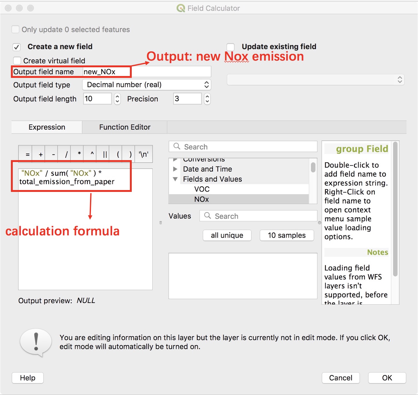
Figure 1. Creating new emission field using field calculator
However, since there are too much point features in this case (1168664 points). The calculating would be extremely slow when GIS processing large shapefile so that it is hardly to get the result using this method without a program crash. Fortunately, there is another trick to do the renormalization instead of using the field calculator directly. We will need to export the shapefile data as spatialite database. The data processing in the format of spatialite database is much faster than it is in shapefile, it will still take minutes to calculate due to the large size of data though. To convert the format of the original data, you can right click on the "onroad" shp data in the table of contents window (aka. layer tree) as shown in Figure 2.
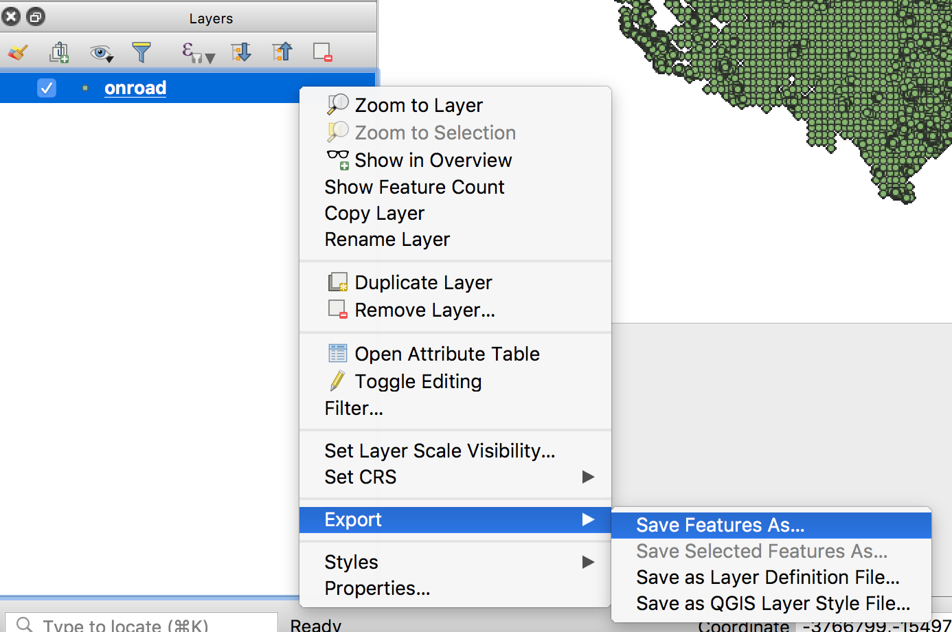
Figure 2. Exporting layer data as SpatiaLite database
In the popped-up window, choose the location you want to save your spatialite data. The on-road data contains varieties of pollutant's concentration. Since many of them are ones will not be used, it would be better to delete some of them. In this study, only the emission of NOx is required so that other fields will be deleted. You can do this in the "Save vector layer as…" window by selecting fields to be exported.
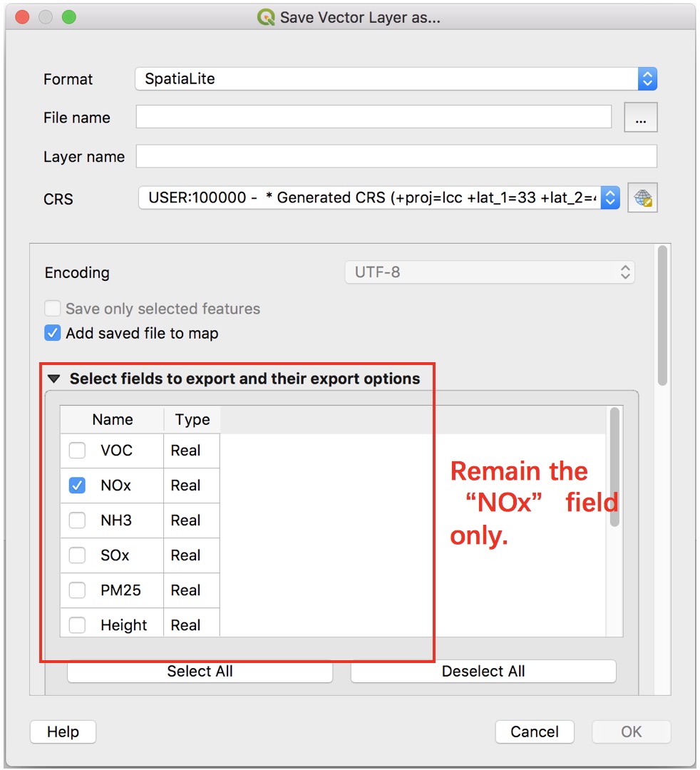
Figure 3. Saving layer options
Alternatively, you can also delete redundant fields in the properties window of the layer file. As shown in Figure 4, in the source filed bar, click "Toggle editing mode" button first. Then choose the fields you intend to delete and click "Delete field" button to remove it.
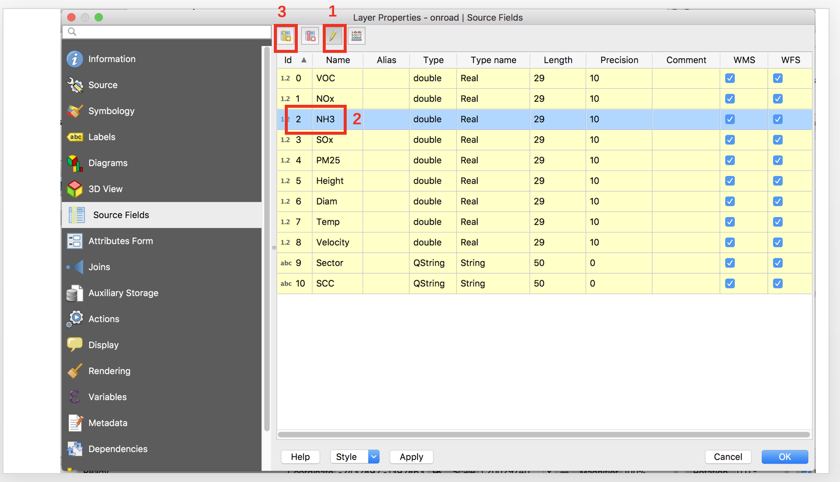
Figure 4. Removing fields in properties window
After the onroad emission data is converted, we may now use the calculator to create the renormalized emission in the opened ".sqlite" file. What should also be mentioned here is that do not use the field calculator with the attribute table open, which would also significantly decrease the running speed. Otherwise, the QGIS will have a great chance to crash. Recall that the unit of the data from the paper is ktonnes/year, which is not one of the input unit values that InMAP supports. So it is important to convert to the appropriate unit when calculating. You would need to repeat the last step, the standardizing, for eight times to get the feasible input data of each year between 2008-2015.
Don't forget that the appropriate format of InMAP model input is shapefile. Therefore, after creating the spatialite data, it is important to convert them back to shapefile format. The final version of data for InMAP model input would be eight standardized shapefiles. In this study, the data used is official published dataset without incorrect data or "NULL" data. If you intend to run the InMAP model with your own data in the future, some data cleaning may be needed.
3. Getting Started with InMAP
You can install InMAP by following the instructions here.
4. Modeling
4.1 Configuration
The first step of setting up an InMAP model simulation is to configure the emission scenario. Emissions files should be in shapefile format where the attribute columns correspond to the names of emitted pollutants. The acceptable pollutant names are VOC, NOx, NH3, SOx, and PM2_5. The model can handle multiple input files, for example, the shapefiles of different elevation. In this case, we only concern the ground level emission.
Then make a copy of the configuration file template and you are going to edit it to meet our scenario condition. The interface of the configuration file should be like below (Figure 5). As seen in the interface, there are a series of parameters you can determine. First, set the evaldata environment variable to the directory you downloaded the evaluation data to, or replace all instances of ${evaldata} in the configuration file with the path to that directory. You must also ensure that the directory OutputFile is to go in exists. Second, choose an emission unit of the input. It should be consistent with the unit in your emission shapefile. Next, set the path of the output file and the log file. Finally, you can look at the output variables (Figure 6) to see which are the output you want to generate. Details about the built-in and calculated variables can be found here.
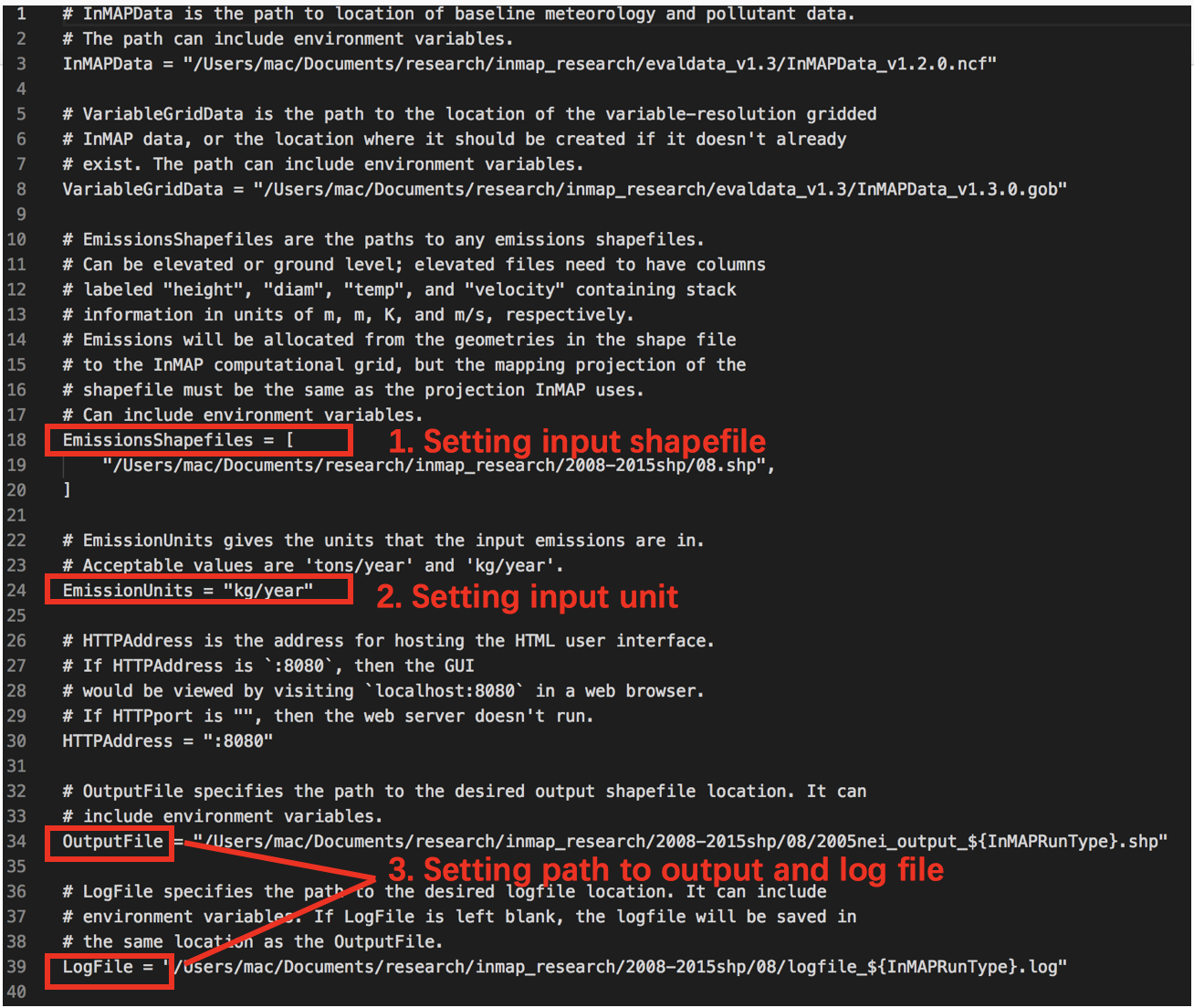
Figure 5. Model Configuration (1)
4.2 Running InMAP
Now you are all set to run the model, using the command below:
inmapX.X.X run steady -s --config=/path/to/configfile.toml
where inmapX.X.X is the name of the executable binary file you have downloaded or compiled on your system. Refer here for more information.
InMAP can run with either a static or dynamically changing grid. Depending on the simulation being run and the configuration settings being used, one or the other grid type may work best; refer here for further discussion. For this tutorial, we will use the static grid as specified by the -s flag above.
You should model the health impact year by year for total 8 times to get the output from 2008-2015.
5. Results and post-processing
5.1 Post-processing
The raw output would be like figure 7 below, taking the 2008 data as an example.
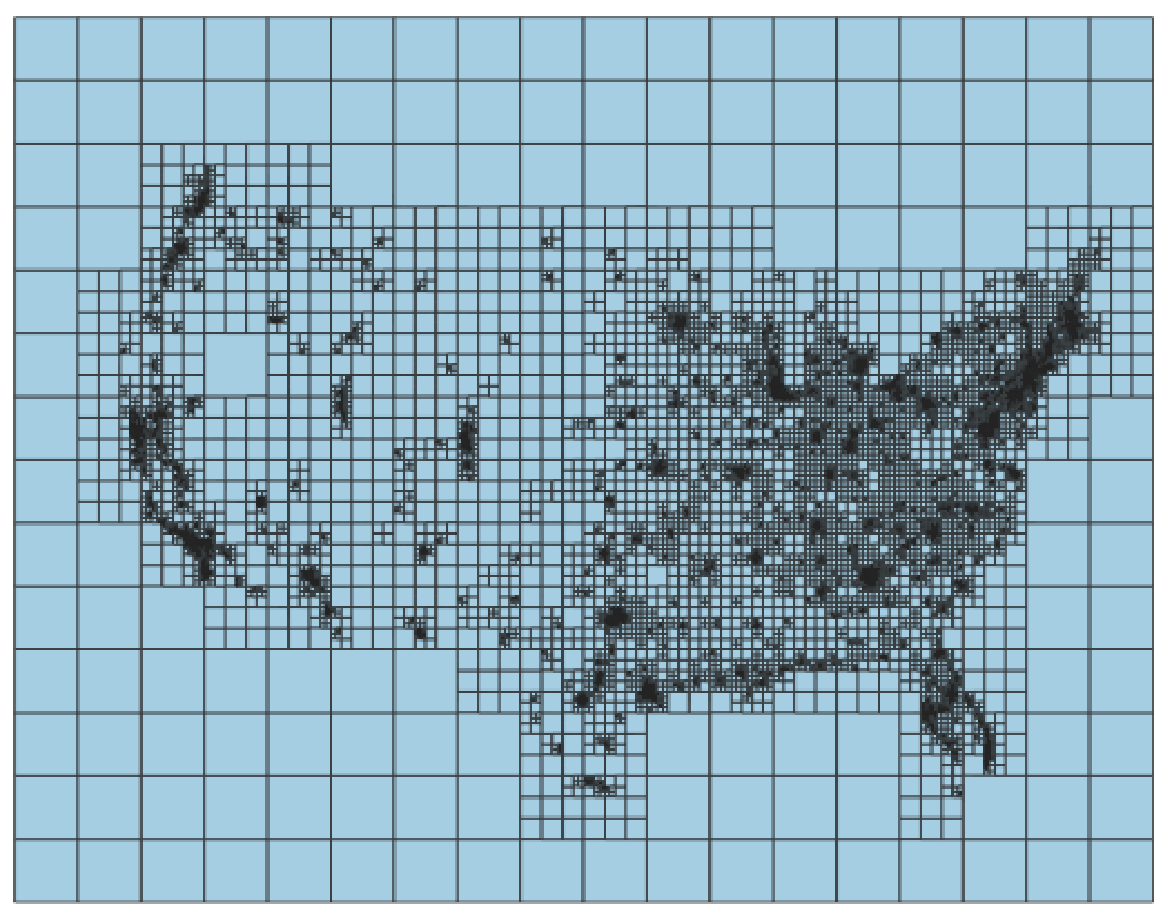
Figure 7. An InMAP output shapefile
Open the attribute table to see all the desired variables we have. We will focus on the "TotalPM25" field.
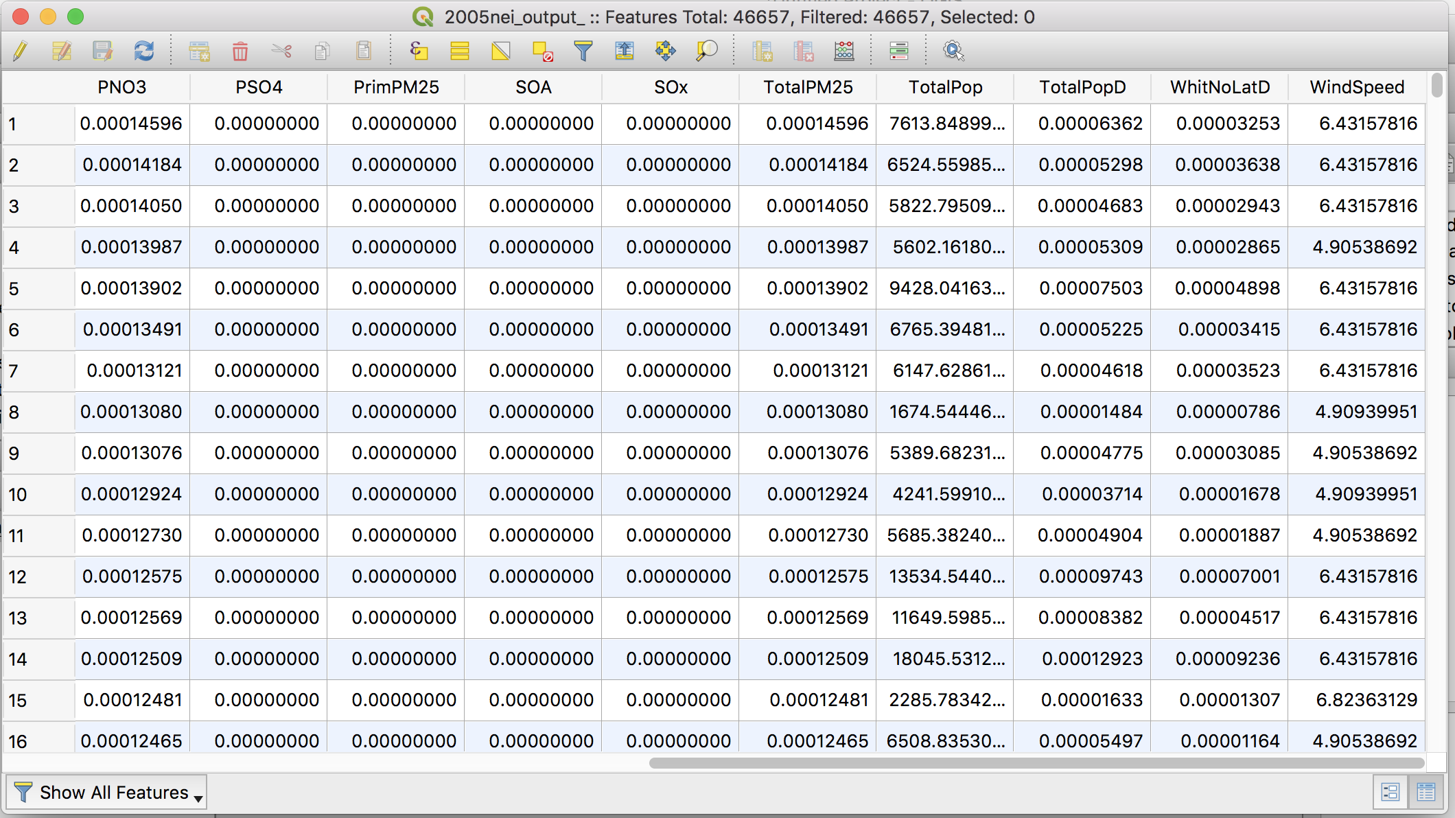
Figure 8. Attribute table of the 2008 output
The features are not symbolized correctly yet. We cannot tell any useful information from the raw output map. Now we are going to make the output more visual. In the menu bar, go to Vector -> Geometry tools -> Centroids. Setting the input layer to your output shapefile and run the tool. After this is accomplished, there will be a new layer in the table of contents, which is a point layer that could be symbolled as a heatmap. Open the properties window of the new layer, choose heatmap as its symbol, set other options as below.
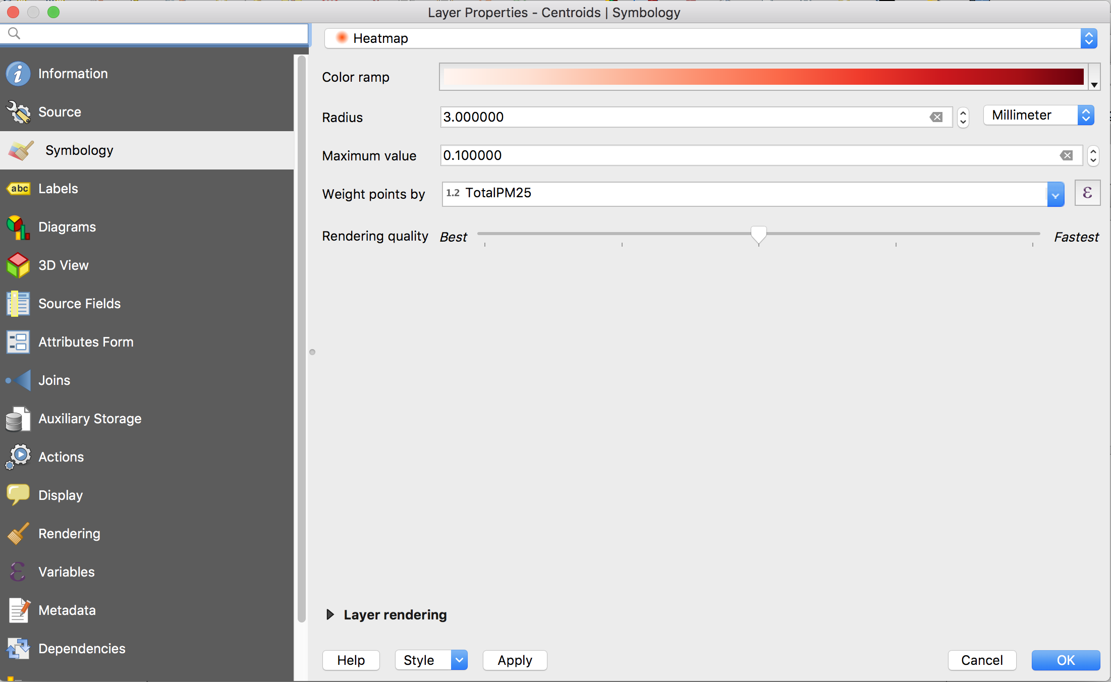
Figure 9. Options for heatmap

Figure 10. Heatmap for total PM2.5
Now the heatmap has been created successfully. But it is still hard to tell the areas with high exposure level belong to which part of U.S. So you need a U.S. states boundary map which you can download here:
https://www.arcgis.com/home/item.html?id=f7f805eb65eb4ab787a0a3e1116ca7e5. Open it and move this layer above the heatmap layer. In the properties window, set the fill color to transparent.
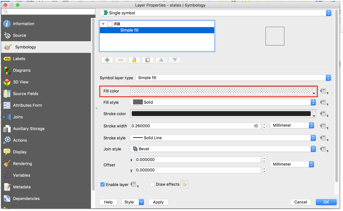
Figure 11. Symbolizing the boundary of the state
Your map now should look like this:
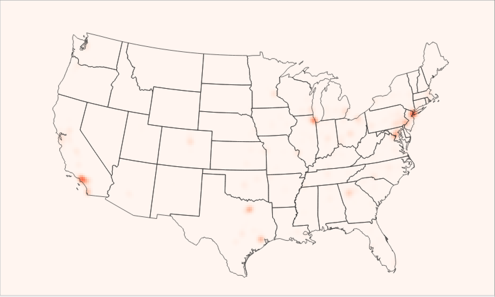
Figure 12. Improved output map
Put the outputs from 2008 to 2015 together to see the variation:
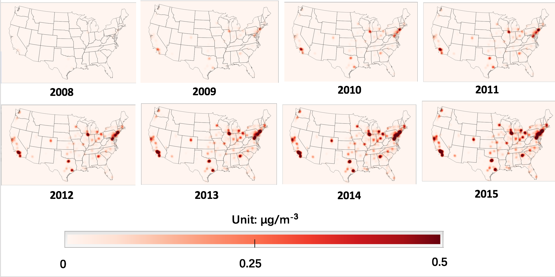
Figure 13. Total PM2.5 from 2008 to 2015
5.2 Compare with Existing Studies
There has been some previous research on the health impacts of the excess emissions caused by the VW defeat devices. Barrett et al. (2015)2 and Holland et al. (2015)3 published estimates of additional emissions of NOx and subsequent health damages due to the using of defeat devices committed by Volkswagen Group in the USA. And Oldenkamp et al. (2016)5 further considered the damages due to ozone formation in addition to PM2.5. We can compare our results with theirs. First, we export each output data to the format of CSV. The data processing is much faster in excel than it is in QGIS. We are interested in the comparison of the total early death from 2008 to 2015 between our model and theirs. So we need to calculate the sum of "TotalPopD" field for each year then sum them together. Table 2 shows the comparison of our result and one from other researches.
Table 2. The comparison of early deaths among studies. (\*95% confidence interval in brackets)
| Studies | Total emissions (ktonnes) | Early deaths (incidences) |
|---|---|---|
| This study | 36.7 (Data from Barrett el al.) | 85.2 |
| Barrett et al. (2015) | 36.7 (12.3-61.2)* | 59 (9.7-150)* |
| Holland et al. (2015) | 45.1 | 46.1 |
| Rik et al. (2016) | 33.8 | 59.2 |
5.3 Conclusion
Our analysis provides an estimate of the public health consequences caused by the additional emissions from Volkswagen defeat devices. The result shows an increase in PM2.5 over time and a spatial distribution that the higher exposure concentration appears at the Eastern and Western coast, Midwest, and Texas. According to the output, there would be average 85 deaths in the U.S.A from 2008 to 2015 due to the extra emission, which is similar to the findings of the previous studies.
References
1Wikipedia contributors. (2018, December 6). Volkswagen emissions scandal. In Wikipedia, The Free Encyclopedia. Retrieved December 13, 2018, from https://en.wikipedia.org/w/index.php?title=Volkswagen_emissions_scandal&oldid=872379047
2Barrett, S. R., Speth, R. L., Eastham, S. D., Dedoussi, I. C., Ashok, A., Malina, R., & Keith, D. W. (2015). Impact of the Volkswagen emissions control defeat device on US public health. Environmental Research Letters, 10(11), 114005.
3Holland, S. P., Mansur, E. T., Muller, N. Z., & Yates, A. J. (2016). Response to Comment on "Damages and expected deaths due to excess NO x emissions from 2009–2015 Volkswagen diesel vehicles". Environmental science & technology, 50(7), 4137-4138.
4Tessum, C. W., Hill, J. D., & Marshall, J. D. (2017). InMAP: A model for air pollution interventions. PloS one, 12(4), e0176131.
5Oldenkamp, R., van Zelm, R., & Huijbregts, M. A. (2016). Valuing the human health damage caused by the fraud of Volkswagen. Environmental Pollution, 212, 121-127.
